2. Train FCN on Pascal VOC Dataset

This is a semantic segmentation tutorial using Gluon Vison, a step-by-step example. The readers should have basic knowledge of deep learning and should be familiar with Gluon API. New users may first go through A 60-minute Gluon Crash Course. You can Start Training Now or Dive into Deep.

Start Training Now

Hint

Feel free to skip the tutorial because the training script is self-complete and ready to launch.

Download Full Python Script: train.py

Example training command:

# First training on augmented set
CUDA_VISIBLE_DEVICES=0,1,2,3 python train.py --dataset pascal_aug --model fcn --backbone resnet50 --lr 0.001 --checkname mycheckpoint
# Finetuning on original set
CUDA_VISIBLE_DEVICES=0,1,2,3 python train.py --dataset pascal_voc --model fcn --backbone resnet50 --lr 0.0001 --checkname mycheckpoint --resume runs/pascal_aug/fcn/mycheckpoint/checkpoint.params

For more training command options, please run python train.py -h Please checkout the model_zoo for training commands of reproducing the pretrained model.

Dive into Deep

import numpy as np
import mxnet as mx
from mxnet import gluon, autograd

import gluoncv

Fully Convolutional Network

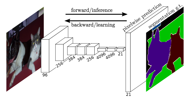
(figure redit to Long et al. )

State-of-the-art approaches of semantic segmentation are typically based on Fully Convolutional Network (FCN) [Long15]. The key idea of a fully convolutional network is that it is “fully convolutional”, which means it does have any fully connected layers. Therefore, the network can accept arbitrary input size and make dense per-pixel predictions. Base/Encoder network is typically pre-trained on ImageNet, because the features learned from diverse set of images contain rich contextual information, which can be beneficial for semantic segmentation.

Model Dilation

The adaption of base network pre-trained on ImageNet leads to loss spatial resolution, because these networks are originally designed for classification task. Following standard implementation in recent works of semantic segmentation, we apply dilation strategy to the stage 3 and stage 4 of the pre-trained networks, which produces stride of 8 featuremaps (models are provided in gluoncv.model_zoo.dilatedresnetv0.DilatedResNetV0). Visualization of dilated/atrous convoution (figure credit to conv_arithmetic ):

Loading a dilated ResNet50 is simply:

pretrained_net = gluoncv.model_zoo.dilatedresnetv0.dilated_resnet50(pretrained=True)

For convenience, we provide a base model for semantic segmentation, which automatically load the pre-trained dilated ResNet gluoncv.model_zoo.SegBaseModel with a convenient method base_forward(input) to get stage 3 & 4 featuremaps:

basemodel = gluoncv.model_zoo.SegBaseModel(nclass=10, aux=False)
x = mx.nd.random.uniform(shape=(1, 3, 224, 224))
c3, c4 = basemodel.base_forward(x)
print('Shapes of c3 & c4 featuremaps are ', c3.shape, c4.shape)

Out:

Shapes of c3 & c4 featuremaps are  (1, 1024, 28, 28) (1, 2048, 28, 28)

FCN Model

We build a fully convolutional “head” on top of the base network, the FCNHead is defined as:

class _FCNHead(HybridBlock):
    def __init__(self, in_channels, channels, norm_layer, **kwargs):
        super(_FCNHead, self).__init__()
        with self.name_scope():
            self.block = nn.HybridSequential()
            inter_channels = in_channels // 4
            with self.block.name_scope():
                self.block.add(nn.Conv2D(in_channels=in_channels, channels=inter_channels,
                                         kernel_size=3, padding=1))
                self.block.add(norm_layer(in_channels=inter_channels))
                self.block.add(nn.Activation('relu'))
                self.block.add(nn.Dropout(0.1))
                self.block.add(nn.Conv2D(in_channels=inter_channels, channels=channels,
                                         kernel_size=1))

def hybrid_forward(self, F, x):
    return self.block(x)

FCN model is provided in gluoncv.model_zoo.FCN. To get FCN model using ResNet50 base network for Pascal VOC dataset:

model = gluoncv.model_zoo.get_fcn(dataset='pascal_voc', backbone='resnet50', pretrained=False)
print(model)

Out:

FCN(
  (conv1): Conv2D(3 -> 64, kernel_size=(7, 7), stride=(2, 2), padding=(3, 3), bias=False)
  (bn1): BatchNorm(axis=1, eps=1e-05, momentum=0.9, fix_gamma=False, use_global_stats=False, in_channels=64)
  (relu): Activation(relu)
  (maxpool): MaxPool2D(size=(3, 3), stride=(2, 2), padding=(1, 1), ceil_mode=False)
  (layer1): HybridSequential(
    (0): DilatedBottleneckV0(
      (conv1): Conv2D(64 -> 64, kernel_size=(1, 1), stride=(1, 1), bias=False)
      (bn1): BatchNorm(axis=1, eps=1e-05, momentum=0.9, fix_gamma=False, use_global_stats=False, in_channels=64)
      (conv2): Conv2D(64 -> 64, kernel_size=(3, 3), stride=(1, 1), padding=(1, 1), bias=False)
      (bn2): BatchNorm(axis=1, eps=1e-05, momentum=0.9, fix_gamma=False, use_global_stats=False, in_channels=64)
      (conv3): Conv2D(64 -> 256, kernel_size=(1, 1), stride=(1, 1), bias=False)
      (bn3): BatchNorm(axis=1, eps=1e-05, momentum=0.9, fix_gamma=False, use_global_stats=False, in_channels=256)
      (relu): Activation(relu)
      (downsample): HybridSequential(
        (0): Conv2D(64 -> 256, kernel_size=(1, 1), stride=(1, 1), bias=False)
        (1): BatchNorm(axis=1, eps=1e-05, momentum=0.9, fix_gamma=False, use_global_stats=False, in_channels=256)
      )
    )
    (1): DilatedBottleneckV0(
      (conv1): Conv2D(256 -> 64, kernel_size=(1, 1), stride=(1, 1), bias=False)
      (bn1): BatchNorm(axis=1, eps=1e-05, momentum=0.9, fix_gamma=False, use_global_stats=False, in_channels=64)
      (conv2): Conv2D(64 -> 64, kernel_size=(3, 3), stride=(1, 1), padding=(1, 1), bias=False)
      (bn2): BatchNorm(axis=1, eps=1e-05, momentum=0.9, fix_gamma=False, use_global_stats=False, in_channels=64)
      (conv3): Conv2D(64 -> 256, kernel_size=(1, 1), stride=(1, 1), bias=False)
      (bn3): BatchNorm(axis=1, eps=1e-05, momentum=0.9, fix_gamma=False, use_global_stats=False, in_channels=256)
      (relu): Activation(relu)
    )
    (2): DilatedBottleneckV0(
      (conv1): Conv2D(256 -> 64, kernel_size=(1, 1), stride=(1, 1), bias=False)
      (bn1): BatchNorm(axis=1, eps=1e-05, momentum=0.9, fix_gamma=False, use_global_stats=False, in_channels=64)
      (conv2): Conv2D(64 -> 64, kernel_size=(3, 3), stride=(1, 1), padding=(1, 1), bias=False)
      (bn2): BatchNorm(axis=1, eps=1e-05, momentum=0.9, fix_gamma=False, use_global_stats=False, in_channels=64)
      (conv3): Conv2D(64 -> 256, kernel_size=(1, 1), stride=(1, 1), bias=False)
      (bn3): BatchNorm(axis=1, eps=1e-05, momentum=0.9, fix_gamma=False, use_global_stats=False, in_channels=256)
      (relu): Activation(relu)
    )
  )
  (layer2): HybridSequential(
    (0): DilatedBottleneckV0(
      (conv1): Conv2D(256 -> 128, kernel_size=(1, 1), stride=(1, 1), bias=False)
      (bn1): BatchNorm(axis=1, eps=1e-05, momentum=0.9, fix_gamma=False, use_global_stats=False, in_channels=128)
      (conv2): Conv2D(128 -> 128, kernel_size=(3, 3), stride=(2, 2), padding=(1, 1), bias=False)
      (bn2): BatchNorm(axis=1, eps=1e-05, momentum=0.9, fix_gamma=False, use_global_stats=False, in_channels=128)
      (conv3): Conv2D(128 -> 512, kernel_size=(1, 1), stride=(1, 1), bias=False)
      (bn3): BatchNorm(axis=1, eps=1e-05, momentum=0.9, fix_gamma=False, use_global_stats=False, in_channels=512)
      (relu): Activation(relu)
      (downsample): HybridSequential(
        (0): Conv2D(256 -> 512, kernel_size=(1, 1), stride=(2, 2), bias=False)
        (1): BatchNorm(axis=1, eps=1e-05, momentum=0.9, fix_gamma=False, use_global_stats=False, in_channels=512)
      )
    )
    (1): DilatedBottleneckV0(
      (conv1): Conv2D(512 -> 128, kernel_size=(1, 1), stride=(1, 1), bias=False)
      (bn1): BatchNorm(axis=1, eps=1e-05, momentum=0.9, fix_gamma=False, use_global_stats=False, in_channels=128)
      (conv2): Conv2D(128 -> 128, kernel_size=(3, 3), stride=(1, 1), padding=(1, 1), bias=False)
      (bn2): BatchNorm(axis=1, eps=1e-05, momentum=0.9, fix_gamma=False, use_global_stats=False, in_channels=128)
      (conv3): Conv2D(128 -> 512, kernel_size=(1, 1), stride=(1, 1), bias=False)
      (bn3): BatchNorm(axis=1, eps=1e-05, momentum=0.9, fix_gamma=False, use_global_stats=False, in_channels=512)
      (relu): Activation(relu)
    )
    (2): DilatedBottleneckV0(
      (conv1): Conv2D(512 -> 128, kernel_size=(1, 1), stride=(1, 1), bias=False)
      (bn1): BatchNorm(axis=1, eps=1e-05, momentum=0.9, fix_gamma=False, use_global_stats=False, in_channels=128)
      (conv2): Conv2D(128 -> 128, kernel_size=(3, 3), stride=(1, 1), padding=(1, 1), bias=False)
      (bn2): BatchNorm(axis=1, eps=1e-05, momentum=0.9, fix_gamma=False, use_global_stats=False, in_channels=128)
      (conv3): Conv2D(128 -> 512, kernel_size=(1, 1), stride=(1, 1), bias=False)
      (bn3): BatchNorm(axis=1, eps=1e-05, momentum=0.9, fix_gamma=False, use_global_stats=False, in_channels=512)
      (relu): Activation(relu)
    )
    (3): DilatedBottleneckV0(
      (conv1): Conv2D(512 -> 128, kernel_size=(1, 1), stride=(1, 1), bias=False)
      (bn1): BatchNorm(axis=1, eps=1e-05, momentum=0.9, fix_gamma=False, use_global_stats=False, in_channels=128)
      (conv2): Conv2D(128 -> 128, kernel_size=(3, 3), stride=(1, 1), padding=(1, 1), bias=False)
      (bn2): BatchNorm(axis=1, eps=1e-05, momentum=0.9, fix_gamma=False, use_global_stats=False, in_channels=128)
      (conv3): Conv2D(128 -> 512, kernel_size=(1, 1), stride=(1, 1), bias=False)
      (bn3): BatchNorm(axis=1, eps=1e-05, momentum=0.9, fix_gamma=False, use_global_stats=False, in_channels=512)
      (relu): Activation(relu)
    )
  )
  (layer3): HybridSequential(
    (0): DilatedBottleneckV0(
      (conv1): Conv2D(512 -> 256, kernel_size=(1, 1), stride=(1, 1), bias=False)
      (bn1): BatchNorm(axis=1, eps=1e-05, momentum=0.9, fix_gamma=False, use_global_stats=False, in_channels=256)
      (conv2): Conv2D(256 -> 256, kernel_size=(3, 3), stride=(1, 1), padding=(1, 1), bias=False)
      (bn2): BatchNorm(axis=1, eps=1e-05, momentum=0.9, fix_gamma=False, use_global_stats=False, in_channels=256)
      (conv3): Conv2D(256 -> 1024, kernel_size=(1, 1), stride=(1, 1), bias=False)
      (bn3): BatchNorm(axis=1, eps=1e-05, momentum=0.9, fix_gamma=False, use_global_stats=False, in_channels=1024)
      (relu): Activation(relu)
      (downsample): HybridSequential(
        (0): Conv2D(512 -> 1024, kernel_size=(1, 1), stride=(1, 1), bias=False)
        (1): BatchNorm(axis=1, eps=1e-05, momentum=0.9, fix_gamma=False, use_global_stats=False, in_channels=1024)
      )
    )
    (1): DilatedBottleneckV0(
      (conv1): Conv2D(1024 -> 256, kernel_size=(1, 1), stride=(1, 1), bias=False)
      (bn1): BatchNorm(axis=1, eps=1e-05, momentum=0.9, fix_gamma=False, use_global_stats=False, in_channels=256)
      (conv2): Conv2D(256 -> 256, kernel_size=(3, 3), stride=(1, 1), padding=(2, 2), dilation=(2, 2), bias=False)
      (bn2): BatchNorm(axis=1, eps=1e-05, momentum=0.9, fix_gamma=False, use_global_stats=False, in_channels=256)
      (conv3): Conv2D(256 -> 1024, kernel_size=(1, 1), stride=(1, 1), bias=False)
      (bn3): BatchNorm(axis=1, eps=1e-05, momentum=0.9, fix_gamma=False, use_global_stats=False, in_channels=1024)
      (relu): Activation(relu)
    )
    (2): DilatedBottleneckV0(
      (conv1): Conv2D(1024 -> 256, kernel_size=(1, 1), stride=(1, 1), bias=False)
      (bn1): BatchNorm(axis=1, eps=1e-05, momentum=0.9, fix_gamma=False, use_global_stats=False, in_channels=256)
      (conv2): Conv2D(256 -> 256, kernel_size=(3, 3), stride=(1, 1), padding=(2, 2), dilation=(2, 2), bias=False)
      (bn2): BatchNorm(axis=1, eps=1e-05, momentum=0.9, fix_gamma=False, use_global_stats=False, in_channels=256)
      (conv3): Conv2D(256 -> 1024, kernel_size=(1, 1), stride=(1, 1), bias=False)
      (bn3): BatchNorm(axis=1, eps=1e-05, momentum=0.9, fix_gamma=False, use_global_stats=False, in_channels=1024)
      (relu): Activation(relu)
    )
    (3): DilatedBottleneckV0(
      (conv1): Conv2D(1024 -> 256, kernel_size=(1, 1), stride=(1, 1), bias=False)
      (bn1): BatchNorm(axis=1, eps=1e-05, momentum=0.9, fix_gamma=False, use_global_stats=False, in_channels=256)
      (conv2): Conv2D(256 -> 256, kernel_size=(3, 3), stride=(1, 1), padding=(2, 2), dilation=(2, 2), bias=False)
      (bn2): BatchNorm(axis=1, eps=1e-05, momentum=0.9, fix_gamma=False, use_global_stats=False, in_channels=256)
      (conv3): Conv2D(256 -> 1024, kernel_size=(1, 1), stride=(1, 1), bias=False)
      (bn3): BatchNorm(axis=1, eps=1e-05, momentum=0.9, fix_gamma=False, use_global_stats=False, in_channels=1024)
      (relu): Activation(relu)
    )
    (4): DilatedBottleneckV0(
      (conv1): Conv2D(1024 -> 256, kernel_size=(1, 1), stride=(1, 1), bias=False)
      (bn1): BatchNorm(axis=1, eps=1e-05, momentum=0.9, fix_gamma=False, use_global_stats=False, in_channels=256)
      (conv2): Conv2D(256 -> 256, kernel_size=(3, 3), stride=(1, 1), padding=(2, 2), dilation=(2, 2), bias=False)
      (bn2): BatchNorm(axis=1, eps=1e-05, momentum=0.9, fix_gamma=False, use_global_stats=False, in_channels=256)
      (conv3): Conv2D(256 -> 1024, kernel_size=(1, 1), stride=(1, 1), bias=False)
      (bn3): BatchNorm(axis=1, eps=1e-05, momentum=0.9, fix_gamma=False, use_global_stats=False, in_channels=1024)
      (relu): Activation(relu)
    )
    (5): DilatedBottleneckV0(
      (conv1): Conv2D(1024 -> 256, kernel_size=(1, 1), stride=(1, 1), bias=False)
      (bn1): BatchNorm(axis=1, eps=1e-05, momentum=0.9, fix_gamma=False, use_global_stats=False, in_channels=256)
      (conv2): Conv2D(256 -> 256, kernel_size=(3, 3), stride=(1, 1), padding=(2, 2), dilation=(2, 2), bias=False)
      (bn2): BatchNorm(axis=1, eps=1e-05, momentum=0.9, fix_gamma=False, use_global_stats=False, in_channels=256)
      (conv3): Conv2D(256 -> 1024, kernel_size=(1, 1), stride=(1, 1), bias=False)
      (bn3): BatchNorm(axis=1, eps=1e-05, momentum=0.9, fix_gamma=False, use_global_stats=False, in_channels=1024)
      (relu): Activation(relu)
    )
  )
  (layer4): HybridSequential(
    (0): DilatedBottleneckV0(
      (conv1): Conv2D(1024 -> 512, kernel_size=(1, 1), stride=(1, 1), bias=False)
      (bn1): BatchNorm(axis=1, eps=1e-05, momentum=0.9, fix_gamma=False, use_global_stats=False, in_channels=512)
      (conv2): Conv2D(512 -> 512, kernel_size=(3, 3), stride=(1, 1), padding=(2, 2), dilation=(2, 2), bias=False)
      (bn2): BatchNorm(axis=1, eps=1e-05, momentum=0.9, fix_gamma=False, use_global_stats=False, in_channels=512)
      (conv3): Conv2D(512 -> 2048, kernel_size=(1, 1), stride=(1, 1), bias=False)
      (bn3): BatchNorm(axis=1, eps=1e-05, momentum=0.9, fix_gamma=False, use_global_stats=False, in_channels=2048)
      (relu): Activation(relu)
      (downsample): HybridSequential(
        (0): Conv2D(1024 -> 2048, kernel_size=(1, 1), stride=(1, 1), bias=False)
        (1): BatchNorm(axis=1, eps=1e-05, momentum=0.9, fix_gamma=False, use_global_stats=False, in_channels=2048)
      )
    )
    (1): DilatedBottleneckV0(
      (conv1): Conv2D(2048 -> 512, kernel_size=(1, 1), stride=(1, 1), bias=False)
      (bn1): BatchNorm(axis=1, eps=1e-05, momentum=0.9, fix_gamma=False, use_global_stats=False, in_channels=512)
      (conv2): Conv2D(512 -> 512, kernel_size=(3, 3), stride=(1, 1), padding=(4, 4), dilation=(4, 4), bias=False)
      (bn2): BatchNorm(axis=1, eps=1e-05, momentum=0.9, fix_gamma=False, use_global_stats=False, in_channels=512)
      (conv3): Conv2D(512 -> 2048, kernel_size=(1, 1), stride=(1, 1), bias=False)
      (bn3): BatchNorm(axis=1, eps=1e-05, momentum=0.9, fix_gamma=False, use_global_stats=False, in_channels=2048)
      (relu): Activation(relu)
    )
    (2): DilatedBottleneckV0(
      (conv1): Conv2D(2048 -> 512, kernel_size=(1, 1), stride=(1, 1), bias=False)
      (bn1): BatchNorm(axis=1, eps=1e-05, momentum=0.9, fix_gamma=False, use_global_stats=False, in_channels=512)
      (conv2): Conv2D(512 -> 512, kernel_size=(3, 3), stride=(1, 1), padding=(4, 4), dilation=(4, 4), bias=False)
      (bn2): BatchNorm(axis=1, eps=1e-05, momentum=0.9, fix_gamma=False, use_global_stats=False, in_channels=512)
      (conv3): Conv2D(512 -> 2048, kernel_size=(1, 1), stride=(1, 1), bias=False)
      (bn3): BatchNorm(axis=1, eps=1e-05, momentum=0.9, fix_gamma=False, use_global_stats=False, in_channels=2048)
      (relu): Activation(relu)
    )
  )
  (head): _FCNHead(
    (block): HybridSequential(
      (0): Conv2D(2048 -> 512, kernel_size=(3, 3), stride=(1, 1), padding=(1, 1))
      (1): BatchNorm(axis=1, eps=1e-05, momentum=0.9, fix_gamma=False, use_global_stats=False, in_channels=512)
      (2): Activation(relu)
      (3): Dropout(p = 0.1, axes=())
      (4): Conv2D(512 -> 22, kernel_size=(1, 1), stride=(1, 1))
    )
  )
  (auxlayer): _FCNHead(
    (block): HybridSequential(
      (0): Conv2D(1024 -> 256, kernel_size=(3, 3), stride=(1, 1), padding=(1, 1))
      (1): BatchNorm(axis=1, eps=1e-05, momentum=0.9, fix_gamma=False, use_global_stats=False, in_channels=256)
      (2): Activation(relu)
      (3): Dropout(p = 0.1, axes=())
      (4): Conv2D(256 -> 22, kernel_size=(1, 1), stride=(1, 1))
    )
  )
)

Dataset and Data Augmentation

image transform for color normalization

from mxnet.gluon.data.vision import transforms
input_transform = transforms.Compose([
    transforms.ToTensor(),
    transforms.Normalize([.485, .456, .406], [.229, .224, .225]),
])

We provide semantic segmentation datasets in gluoncv.data. For example, we can easily get the Pascal VOC 2012 dataset:

trainset = gluoncv.data.VOCSegmentation(split='train', transform=input_transform)
print('Training images:', len(trainset))
# Create Training Loader
train_data = gluon.data.DataLoader(
    trainset, 4, shuffle=True, last_batch='rollover',
    num_workers=4)

Out:

Training images: 2913

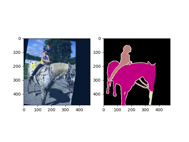
For data augmentation, we follow the standard data augmentation routine to transform the input image and the ground truth label map synchronously. (Note that “nearest” mode upsample are applied to the label maps to avoid messing up the boundaries.) We first randomly scale the input image from 0.5 to 2.0 times, then rotate the image from -10 to 10 degrees, and crop the image with padding if needed. Finally a random Gaussian blurring is applied.

Random pick one example for visualization:

from random import randint
idx = randint(0, len(trainset))
img, mask = trainset[idx]
from gluoncv.utils.viz import get_color_pallete, DeNormalize
# get color pallete for visualize mask
mask = get_color_pallete(mask.asnumpy(), dataset='pascal_voc')
mask.save('mask.png')
# denormalize the image
img = DeNormalize([.485, .456, .406], [.229, .224, .225])(img)
img = np.transpose((img.asnumpy()*255).astype(np.uint8), (1, 2, 0))

Plot the image and mask

from matplotlib import pyplot as plt
import matplotlib.image as mpimg
# subplot 1 for img
fig = plt.figure()
fig.add_subplot(1,2,1)

plt.imshow(img)
# subplot 2 for the mask
mmask = mpimg.imread('mask.png')
fig.add_subplot(1,2,2)
plt.imshow(mmask)
# display
plt.show()

Training Details

• Training Losses:

  We apply a standard per-pixel Softmax Cross Entropy Loss to train FCN. For Pascal VOC dataset, we ignore the loss from boundary class (number 22). Additionally, an Auxiliary Loss as in PSPNet [Zhao17] at Stage 3 can be enabled when training with command --aux. This will create an additional FCN “head” after Stage 3.

from gluoncv.model_zoo.segbase import SoftmaxCrossEntropyLossWithAux
criterion = SoftmaxCrossEntropyLossWithAux(aux=True)

• Learning Rate and Scheduling:

  We use different learning rate for FCN “head” and the base network. For the FCN “head”, we use \(10\times\) base learning rate, because those layers are learned from scratch. We use a poly-like learning rate scheduler for FCN training, provided in gluoncv.utils.PolyLRScheduler. The learning rate is given by \(lr = baselr \times (1-iter)^{power}\)

lr_scheduler = gluoncv.utils.PolyLRScheduler(0.001, niters=len(train_data),
                                                 nepochs=50)

• Dataparallel for multi-gpu training

from gluoncv.utils.parallel import *
ctx_list = [mx.gpu(0), mx.gpu(1)]
model = DataParallelModel(model, ctx_list)
criterion = DataParallelCriterion(criterion, ctx_list)

• Create SGD solver

kv = mx.kv.create('device')
optimizer = gluon.Trainer(model.module.collect_params(), 'sgd',
                          {'lr_scheduler': lr_scheduler,
                           'wd':0.0001,
                           'momentum': 0.9,
                           'multi_precision': True},
                          kvstore = kv)

The training loop

train_loss = 0.0
epoch = 0
for i, (data, target) in enumerate(train_data):
    lr_scheduler.update(i, epoch)
    with autograd.record(True):
        outputs = model(data)
        losses = criterion(outputs, target)
        mx.nd.waitall()
        autograd.backward(losses)
    optimizer.step(4)
    for loss in losses:
        train_loss += loss.asnumpy()[0] / len(losses)
    print('Epoch %d, training loss %.3f'%(epoch, train_loss/(i+1)))
    # just demo for 20 iters
    if i > 20:
        break

Out:

Epoch 0, training loss 4.125
Epoch 0, training loss 3.925
Epoch 0, training loss 3.612
Epoch 0, training loss 3.307
Epoch 0, training loss 3.234
Epoch 0, training loss 2.959
Epoch 0, training loss 2.939
Epoch 0, training loss 2.961
Epoch 0, training loss 2.748
Epoch 0, training loss 2.594
Epoch 0, training loss 2.860
Epoch 0, training loss 2.956
Epoch 0, training loss 2.961
Epoch 0, training loss 2.808
Epoch 0, training loss 2.882
Epoch 0, training loss 2.862
Epoch 0, training loss 2.807
Epoch 0, training loss 2.793
Epoch 0, training loss 2.763
Epoch 0, training loss 2.692
Epoch 0, training loss 2.724
Epoch 0, training loss 2.724

You can Start Training Now.

References

[Long15]

Long, Jonathan, Evan Shelhamer, and Trevor Darrell. “Fully convolutional networks for semantic segmentation.” Proceedings of the IEEE conference on computer vision and pattern recognition. 2015.

[Zhao17]

Zhao, Hengshuang, Jianping Shi, Xiaojuan Qi, Xiaogang Wang, and Jiaya Jia. “Pyramid scene parsing network.” IEEE Conf. on Computer Vision and Pattern Recognition (CVPR). 2017.

Total running time of the script: ( 0 minutes 24.714 seconds)