5. Train Your Own Model on ImageNet

ImageNet is the most well-known dataset for image classification. Since it was published, most of the research that advances the state-of-the-art of image classification was based on this dataset.

Although there are a lot of available models, it is still a non-trivial task to train a state-of-the-art model on ImageNet from scratch. In this tutorial, we will smoothly walk you through the process of training a model on ImageNet.

Note

The rest of the tutorial walks you through the details of ImageNet training. If you want a quick start without knowing the details, try downloading this script and start training with just one command.

Download train_imagenet.py

The commands used to reproduce results from papers are given in our Model Zoo.

Note

Since real training is extremely resource consuming, we don’t actually execute code blocks in this tutorial.

Prerequisites

Expertise

We assume readers have a basic understanding of Gluon, we suggest you start with Gluon Crash Course .

Also, we assume that readers have gone through previous tutorials on CIFAR10 Training and ImageNet Demo .

Data Preparation

Unlike CIFAR10, we need to prepare the data manually. If you haven’t done so, please go through our tutorial on Prepare ImageNet Data .

Hardware

Training deep learning models on a dataset of over one million images is very resource demanding. Two main bottlenecks are tensor computation and data IO.

For tensor computation, it is recommended to use a GPU, preferably a high-end one. Using multiple GPUs together will further reduce training time.

For data IO, we recommend a fast CPU and a SSD disk. Data loading can greatly benefit from multiple CPU threads, and a fast SSD disk. Note that in total the compressed and extracted ImageNet data could occupy around 300GB disk space, thus a SSD with at least 300GB is required.

Network structure

Finished preparation? Let’s get started!

First, import the necessary libraries into python.

import argparse, time

import numpy as np
import mxnet as mx

from mxnet import gluon, nd
from mxnet import autograd as ag
from mxnet.gluon import nn
from mxnet.gluon.data.vision import transforms

from gluoncv.model_zoo import get_model
from gluoncv.utils import makedirs, TrainingHistory

In this tutorial we use ResNet50_v2, a network with balanced prediction accuracy and computational cost.

# number of GPUs to use
num_gpus = 4
ctx = [mx.gpu(i) for i in range(num_gpus)]

# Get the model ResNet50_v2, with 10 output classes
net = get_model('ResNet50_v2', classes=1000)
net.initialize(mx.init.Xavier(magnitude=2), ctx = ctx)

Note that the ResNet model we use here for ImageNet is different in structure from the one we used to train CIFAR10. Please refer to the original paper or GluonCV codebase for details.

Data Augmentation and Data Loader

Data augmentation is essential for a good result. It is similar to what we have in the CIFAR10 training tutorial, just different in the parameters.

We compose our transform functions as following:

jitter_param = 0.4
lighting_param = 0.1

transform_train = transforms.Compose([
    transforms.RandomResizedCrop(224),
    transforms.RandomFlipLeftRight(),
    transforms.RandomColorJitter(brightness=jitter_param, contrast=jitter_param,
                                 saturation=jitter_param),
    transforms.RandomLighting(lighting_param),
    transforms.ToTensor(),
    transforms.Normalize([0.485, 0.456, 0.406], [0.229, 0.224, 0.225])
])

Since ImageNet images have much higher resolution and quality than CIFAR10, we can crop a larger image (224x224) as input to the model.

For prediction, we still need deterministic results. The transform function is:

transform_test = transforms.Compose([
    transforms.Resize(256),
    transforms.CenterCrop(224),
    transforms.ToTensor(),
    transforms.Normalize([0.485, 0.456, 0.406], [0.229, 0.224, 0.225])
])

Notice that it is important to keep the normalization consistent, since trained model only works well on test data from the same distribution.

With the transform functions, we can define data loaders for our training and validation datasets.

# Batch Size for Each GPU
per_device_batch_size = 64
# Number of data loader workers
num_workers = 32
# Calculate effective total batch size
batch_size = per_device_batch_size * num_gpus

data_path = '~/.mxnet/datasets/imagenet'

# Set train=True for training data
# Set shuffle=True to shuffle the training data
train_data = gluon.data.DataLoader(
    imagenet.classification.ImageNet(data_path, train=True).transform_first(transform_train),
    batch_size=batch_size, shuffle=True, last_batch='discard', num_workers=num_workers)

# Set train=False for validation data
val_data = gluon.data.DataLoader(
    imagenet.classification.ImageNet(data_path, train=False).transform_first(transform_test),
    batch_size=batch_size, shuffle=False, num_workers=num_workers)

Note that we set per_device_batch_size=64, which may not suit GPUs with Memory smaller than 12GB. Please tune the value according to your specific configuration.

Path '~/.mxnet/datasets/imagenet' is the default path if you prepared the data with our script.

Optimizer, Loss and Metric

Optimizer is what improves the model during training. We use the popular Nesterov accelerated gradient descent algorithm.

# Learning rate decay factor
lr_decay = 0.1
# Epochs where learning rate decays
lr_decay_epoch = [30, 60, 90, np.inf]

# Nesterov accelerated gradient descent
optimizer = 'nag'
# Set parameters
optimizer_params = {'learning_rate': 0.1, 'wd': 0.0001, 'momentum': 0.9}

# Define our trainer for net
trainer = gluon.Trainer(net.collect_params(), optimizer, optimizer_params)

For classification tasks, we usually use softmax cross entropy as the loss function.

loss_fn = gluon.loss.SoftmaxCrossEntropyLoss()

With 1000 classes the model may not always rate the correct answer with the highest rank. Besides top-1 accuracy, we also consider top-5 accuracy as a measurement of how well the model is doing.

At the end of every epoch, we record and print the metric scores.

acc_top1 = mx.metric.Accuracy()
acc_top5 = mx.metric.TopKAccuracy(5)
train_history = TrainingHistory(['training-top1-err', 'training-top5-err',
                                 'validation-top1-err', 'validation-top5-err'])

Validation

At the end of every training epoch, we evaluate it on the validation data set, and report the top-1 and top-5 error rate.

def test(ctx, val_data):
    acc_top1_val = mx.metric.Accuracy()
    acc_top5_val = mx.metric.TopKAccuracy(5)
    for i, batch in enumerate(val_data):
        data = gluon.utils.split_and_load(batch[0], ctx_list=ctx, batch_axis=0)
        label = gluon.utils.split_and_load(batch[1], ctx_list=ctx, batch_axis=0)
        outputs = [net(X) for X in data]
        acc_top1_val.update(label, outputs)
        acc_top5_val.update(label, outputs)

    _, top1 = acc_top1_val.get()
    _, top5 = acc_top5_val.get()
    return (1 - top1, 1 - top5)

Training

After all these preparation, we can finally start training! Following is the main training loop:

epochs = 120
lr_decay_count = 0
log_interval = 50
num_batch = len(train_data)

for epoch in range(epochs):
    tic = time.time()
    btic = time.time()
    acc_top1.reset()
    acc_top5.reset()
    train_loss = 0

    if lr_decay_period == 0 and epoch == lr_decay_epoch[lr_decay_count]:
        trainer.set_learning_rate(trainer.learning_rate*lr_decay)
        lr_decay_count += 1

    for i, batch in enumerate(train_data):
        data = gluon.utils.split_and_load(batch[0], ctx_list=ctx, batch_axis=0)
        label = gluon.utils.split_and_load(batch[1], ctx_list=ctx, batch_axis=0)
        with ag.record():
            outputs = [net(X) for X in data]
            loss = [L(yhat, y) for yhat, y in zip(outputs, label)]
        for l in loss:
            l.backward()
        trainer.step(batch_size)
        acc_top1.update(label, outputs)
        acc_top5.update(label, outputs)
        train_loss += sum([l.sum().asscalar() for l in loss])
        if log_interval and not (i + 1) % log_interval:
            _, top1 = acc_top1.get()
            _, top5 = acc_top5.get()
            err_top1, err_top5 = (1-top1, 1-top5)
            print('Epoch[%d] Batch [%d]     Speed: %f samples/sec   top1-err=%f     top5-err=%f'%(
                      epoch, i, batch_size*opt.log_interval/(time.time()-btic), err_top1, err_top5))
            btic = time.time()

    _, top1 = acc_top1.get()
    _, top5 = acc_top5.get()
    err_top1, err_top5 = (1-top1, 1-top5)
    train_loss /= num_batch * batch_size

    err_top1_val, err_top5_val = test(ctx, val_data)
    train_history.update([err_top1, err_top5, err_top1_val, err_top5_val])

    print('[Epoch %d] training: err-top1=%f err-top5=%f loss=%f'%(epoch, err_top1, err_top5, train_loss))
    print('[Epoch %d] time cost: %f'%(epoch, time.time()-tic))
    print('[Epoch %d] validation: err-top1=%f err-top5=%f'%(epoch, err_top1_val, err_top5_val))

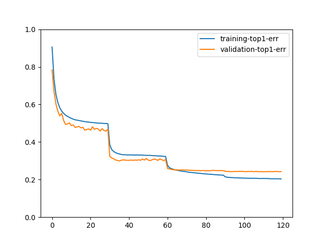
We can plot the top-1 error rates with:

train_history.plot(['training-top1-err', 'validation-top1-err'])

If you train the model with epochs=120, the plot may look like:

Next Step

Model Zoo provides scripts and commands for training models on ImageNet.

If you want to know what you can do with the model you just trained, please read the tutorial on Transfer learning.

Besides classification, deep learning models nowadays can do other exciting tasks like object detection and semantic segmentation.

Total running time of the script: ( 0 minutes 0.000 seconds)